Transformation Matrices

In the previous section, we saw how multiplying a vector by a matrix will give us another vector. Well, as we briefly mentioned before, these matrices can be used to "store" transformations (rotations, scaling, translations). Any vector multiplied by this matrix will result in a new vector which has had these transformations applied. This is where the power of the matrix comes in.

The Identity Matrix

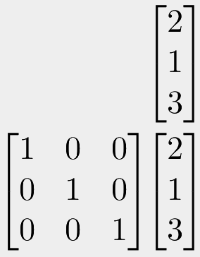
OK so just before we look at transformations, I am going to start off by showing you the identity matrix. An identity matrix is a matrix which doesn't actually do anything. It is the equivalent of multiplying a regular number by 1. The result is always the same as what we started with.

We can see an example of multiplying a vector by an identity matrix below. Notice that if you calculate the multiplication, the output will always be exactly the same as the input.

The key thing about the identity matrix is that it is a square matrix (same number of columns as rows), and that it has only 1's on the diagonal (the technical name for...the diagonal set of numbers top-left to bottom-right). Everywhere else it must have zeroes.

So why does it exist then? What's significant about it?

Well firstly, as it is in effect a "blank" transformation matrix, representing no change, it is often the default value that matrices are initialised to.

Secondly, in our program, our code may iterate over every 3D model and multiply each of its coordinates by a local transformation matrix. This can be useful to make sure everything is scaled correctly, and perhaps some other things. In one particular case, perhaps everything is already scaled correctly. We could write some specific flags and code to not run anything on this model, but these special cases might make our code messy, and require thinking about special cases in different parts of the code. Instead, we can just set our local transform matrix to be the identity matrix. The calculation can still be done, and what goes in will be the same as what goes out.

Scaling

The simplest transformation to think about, besides the identity matrix, is a scaling matrix. It looks like this:

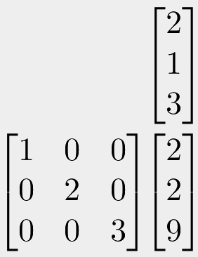
If you consider the step by step process of multiplication, you can see that any 3D coordinate multiplied by this matrix, will have its x value multiplied by one, its y coordinate doubled, and its z coordinate will be multiplied by three. If you do this process step-by-step, you should see why scaling must be performed on the diagonal, and all other values must be zero for this to work. All points in our world that we multiply by this matrix will therefore be scaled by those amounts. We can set pretty much any values for these, to scale by that amount in that axis. Scaling by zero will effectively flatten the world in that axis.

You can also scale an axis by negative values. Setting the top-left value of our scaling matrix to -1 would mean that any input points would become flipped in their x-axis - effectively mirroring them in that axis. You can of course multiply them by -2 to double their size and flip them.

Translations

Translating our input points (adding or subtracting some value to each component of them) might sound simple, but it's actually a little bit trickier. The give away here is in the name - we are performing matrix multiplication, not addition. However there is a nice trick to allow us to bypass this limitation.

If you haven't read up on Homogeneous Coordinates yet, please make sure you do before going further!.

To translate coordinates, we must first extend the length of the vector by adding an extra dimension to it, and setting its value to 1, making it a homogeneous coordinate. As we are now multiplying a 3x3 matrix by a 4x1 vector, we must also increase the size of our matrix to 3x4 to make the multiplication possible. Better yet, if we increase the size of our matrix to 4x4, it will be square, and therefore mean that the result of the multiplication will have the same size as the vector input. Specifically, this will mean the output vector is also homogeneous.

Have a look at the following multiplication:

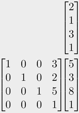
If you work through the matrix multiplication, it should give you a good feeling for why this works. The extra 1 on the input allows us to use the final column of the matrix as the translation vector. As these values are always multiplied by the 1, they remain the same, and because of how matrix multiplications adds between the totals, this result just gets added onto the output.

We can see that each coordinate is multiplied by one, so are not scaled. But the right-most column of the transformation matrix will add 3 to the x coordinate, 2 to the y coordinate, and 5 to the z coordinate.

Thus, we have our translation. We can also see that the bottom row of the transformation matrix multiplies everything else by zero, so the result will always just be 1x1. Therefore the resulting coordinate will always be another homogeneous coordinate with 1 in the final column, so can just be multiplied by further 4x4 transformation matrices without any modification.

To convert it back to a regular coordinate, we can just ignore this final 1. As we mentioned in the section on homogeneous coordinates before though, if you imagine the input coordinate had a zero in the final position, the matrix multiplication would effectively multiply all the translational components in the right-most column by zero and then add them on, so would essentially "ignore" any translations!

If we permanently keep all our 3D coordinates instead as a homogeneous 4x1 vector, where the last value is 1, then they will no longer be multipliable with our scaling matrices. What we can do though is to add an extra column and row to our scaling matrix, which is all zero except 1 in the bottom right. Now, with a 4x4 scaling matrix, 4x4 translation matrix, and 4x1 position vector, everything is neatly compatible. Make your coordinates a 4x1 homogeneous vector, multiply by any combination of 4x4 translations matrices and 4x4 scaling matrices, then when you're done remove the final 1 value in the resulting vector, and you have your new coordinate.

Rotations

Rotations are the final kind of transformation you will use often. Other kinds do exist, like shear transformations, but honestly are used very rarely, and only for funky effects.

Rotations are....a little complicated compared to other kinds of transformations as they involve trigonometry in the matrix. So let's un-complicate things and just look at a 2D world with a 2D coordinate system for now.

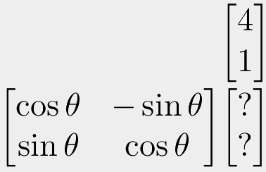
So the first thing you will probably notice is the theta (the symbol which looks something like Θ). This is to be substituted by whatever angle you want to rotate by. Just remember that this needs to be in degrees if you maths functions expect degrees, and radians if they want radians. For now, I will use degrees as most people have a better intuition for them, but you can easily convert from one to the other.

Let's go with an example where we rotate out input coordinate by 90 degrees. So everywhere in our rotation matrix, we replace theta with 90 degrees, and then compute the value. The cosine of 90 degrees is zero, and the sine of it is 1. For completeness, -sine of 90 will get us -1. We can then plug these values into our rotation matrix and calculate the result like normal:

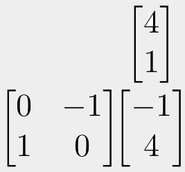
If you plot the position before and after applying the rotation matrix, you will see it has rotated 90 degrees around the origin, in the counter-clockwise direction. Counter-clockwise rotations are the standard for a right-handed coordinate system, which most graphics APIs and mathematics in general use.

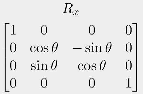
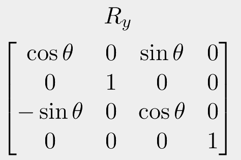
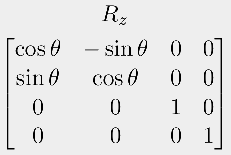
OK, that wasn't too bad. But in 3 dimensions things get complicated. First of all, we will need to switch to a 4x4 matrix to keep things compatible. Worse, in 3D, there are three possible axes to rotate around. Rotating around the x axis has a different result to rotating around the y axis, which means a different transformation matrix.

The good news though, is that things only look complicated. The maths is no different to what you just did.

Also, I want to stress now, you don't need to know these things off the top of your head! Even professionally, these are quickly looked up online each time they need to be used! But it's still a good idea to have an understanding of what they are, how they work, and what they look like.

I'm not going to give a full example here, but to use these, you need to make your input coordinates homogeneous. Then simply choose which 3D axis your points will be rotated around: x, y or z, and use the corresponding matrix. So use the "Rx" matrix to rotate around the x axis. Substitute in your theta angle, compute each value, then just do a regular matrix multiplication.

Combinations

Let's take a moment to consider why matrices are so powerful in the world of graphics. You can take your input vector, and multiply it by the translation matrix to move it around in your world. You can then multiply this transformed position by the scale matrix, and it will be scaled. You can then take the result and multiply it by a rotation matrix, and it will be rotated. Maybe then we multiply it by a final translation matrix to move it around further.

With normal numbers, if you have an equation like 2x5x3x2, you do not have to perform the calculations in any specific order. You can find an easy section, like (2x5)x3x2, solve that, and then simplify the calculation to 10x3x2, and the answer is the same. Well this holds true for matrices too, as long as the overall order does not change.

Instead of multiplying our vector with lots of different transformations one after the other, we can multiply the translation matrix by the scaling matrix to combine them into a single matrix. If they're both 4x4 then the output will also be 4x4. We can then multiply this by the rotation, again 4x4, and then the final translation, again 4x4.

By pre-multiplying these transformation matrices together, we get a resulting matrix of 4x4 which "contains" all the previous transformations, and now any coordinate which is multiplied by this matrix, will be transformed as though each and every step was performed on it individually, and in order.

No matter what convoluted transformations you need to do, and how many of them you need to apply, you just matrix multiply them together to get a single matrix which will do the same thing. No matter how complicated, you will end up with a 4x4 matrix which you can multiply any point with to perform all of those transformations in order in one go.

That's the power of the matrix, and computer hardware (particularly GPUs) can therefore be highly optimised for taking hundreds of thousands of coordinates, and doing a single 4x4 matrix multiplication on them, which will perform all your transformations in one go. This is primarily what the vertex shader does.

One final note about ordering. Usually, or perhaps "unusually", matrix multiplication is performed right-to-left. This isn't just an OpenGL quirk, but applies pretty much universally across mathematics.

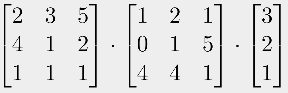
If you consider the above example, we have some 3D point on the right, and two matrices to the left of them. We would work through this calculation by starting with the vector on the right, then multiplying it with the matrix in the middle, then multiplying the result with the matrix on the left. We could also take the middle matrix and "pre-multiply" it with the left-most matrix, giving us a single 3x3 matrix which contains both of these transformations. Then we can multiply the vector by this resulting matrix. Notice that if we do this, we are always multiplying right-with-left.

However, what we cannot do, is to start with the left-most matrix, multiply it with the middle matrix, and then the final vector. Remember, matrix multiplications are non-commutative, so AxB is not the same as BxA. It gives different results. In this case it would lead to you trying to multiply two matrices that have the wrong shapes to be multiplied. So we can only go, and must always go in one direction, either left-to-right, or right-to-left. And because of how we defined matrix multiplication here (the standard way), they only work if we multiply right-to-left.