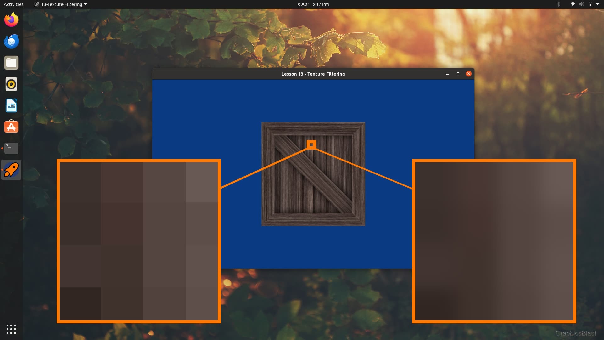
Lesson 13: Texture Filtering

Texture Filtering: We take a deeper look at texture filtering to make our textures look great now matter how they're viewed!

In the previous lesson we implemented texture mapping to breathe some realism into our triangles. One thing we glossed over though is how the texture sampling and filtering process actually works.

Understanding these processes though can make a huge difference to the quality of our final rendered textures, so in this lesson we'll take a detailed look at how texture filtering works, and implement techniques known as mipmapping and anisotropic filtering to make out textures look great on screen.

Sampling

Let's start by looking at what actually happens when we sample a texture.

As we saw in our lesson on the GPU, when we render triangles to our window they will go through a process called rasterisation, which outputs the set of pixels which the triangle occupies on our window. Each of these pixels then has a fragment shader program applied, to figure out the new colour of the pixel.

Let's consider one of these pixels having a fragment shader applied to it. Each of the triangle's three vertices has an associated UV coordinate along with it's regular spatial coordinates. When our fragment shader looks up it's UV coordinate, it will receive a weighted average result based on how close it is to each of the three vertices.

In the simplest possible scenario, when our fragment shader takes this interpolated UV coordinate and a texture, and looks up the texture's colour at that position, it will fall exactly on one of the texture's pixels. In this case, which RGB value the fragment shader should use is clear.

When the fragment shader's UV coordinate does not nicely correspond to an exact pixel in the texture though, but instead somewhere in between some pixels, we have a few strategies open to us to decide how to proceed.

In the previous lesson, we opted for GL_NEAREST as our sampling strategy. This is the most basic setting, and tells our fragment shader to simply grab the RGB data of whichever texture pixel (or "texel") is closest to the UV coordinate we provided. Of course if we look up exactly between two texels, the GPU driver will be forced to choose one of them, usually rounding the UV coordinate up.

On the surface this strategy seems reasonable. But what tends to happen when we use this in the real world is that our textures can end up looking skewed, awkward and pixelated in certain circumstances.

Consider a scenario where our texture contains a distinct vertical line which is only a single texel thick. Well, if it happens that when we render our scene, we end up with fragment shaders being executed either side of this line, and both sides sample the line as their nearest pixel, we can end up with the final rendered image containing the line which is now two pixels thick.

The line from the texture is now overly dominant in the final rendered image, at the expense of other features in the texture. The strategy results in the final image containing a slightly distorted version of the original texture.

Worse still, moving the camera fractionally can change the situation such that now only a single fragment shader "catches" the line as it's nearest texel. The line in the rendered image suddenly becomes much less prominent. This can happen with very small movements of the camera, and causes a flickering effect in the final image known as shimmering.

One way to improve this is to switch to a linearly interpolating sampler. In OpenGL this can be done by simply changing our GL_NEAREST parameter to GL_LINEAR.

A linearly interpolating sampler means that if we try to sample a texture between it's texels, we should instead interpolate between the nearest texels to come up with a weighted average value.

The result of this is a much smoother looking final rendered image. In the above scenario when we sample around a single texel line, instead we'll end up with each pixel being somewhat influenced by the line's RGB values based on how close it is. The final rendered image will be somewhat blurred to fit the misalignment of UV coordinates and texels, which is a much better way to handle these situations than jarring pixelisations of the texture, and our eyes tend to not to notice it as much.

So in this case, why would we ever want to use GL_NEAREST? Why does that code path still exist?

Nope, it's nothing to do with performance! GPU's have been doing linear interpolation of textures for a long time and so the hardware is generally highly optimised to do this.

Well, the reason is that sometimes we don't want to have the blurring associated with the linear interpolation, especially when we're not using a texture for the purpose of texture mapping. We can sometimes use textures to instead indicate specific things to our fragment shader, for example if the texture contains "0", the fragment shader should not calculate something, but if "1" then it should. Ok, a fairly unrealistic example, but the logic is there. This would work fine with GL_NEAREST, but GL_LINEAR would result in a fragment shader on the boundary getting values like 0.6, and the appropriate behaviour might not be clear. Forcing our texture sampler to either pick one texel or another is useful in this case.

It's therefore useful for us to be able to configure our sampling behaviour, but probably a more reasonable default for us to use is GL_LINEAR for a more natural looking image. In OpenGL this can be set for the currently bound texture like this:

glTexParameteri(GL_TEXTURE_2D, GL_TEXTURE_MIN_FILTER, GL_LINEAR);

glTexParameteri(GL_TEXTURE_2D, GL_TEXTURE_MAG_FILTER, GL_LINEAR);

Where here we've used linear interpolation for both the minification and magnification filter (the sampled texels being both larger and smaller than the fragments).

As we encapsulated these functions in our class, we can also set these parameters for our texture objects externally like this:

setParameter(GL_TEXTURE_MIN_FILTER, GL_LINEAR);

setParameter(GL_TEXTURE_MAG_FILTER, GL_LINEAR);

Which will do exactly the same, but makes sure the texture is bound and then updates the parameter.

Edge Sampling Parameters

Related to how we sample between texels is how we sample at the edge of a texture.

If we have a UV coordinate of exactly 1.0 in one of our axes, that tells us we need to look up the colour data at the very outside edge of a texture. However, we have to remember that the texels themselves occupy some physical area. Texels are defined at the centre, so if a texel was positioned at the UV coordinate 1.0, some of it's area would be past the edge of the texture. This is obviously not possible, the outer edge of a texture must be at the outside of a texel, not at it's centre.

Therefore, edge texels must have a UV coordinate of less than one. It must be (well, it's centre must be) somewhere inside the texture. This also applies at the start too - the first texel of an image will not have a UV coordinate of zero, but something greater than zero.

While not a problem if we're using GL_NEAREST as our sampling technique, if we're using GL_LINEAR and sample right at the edge, we need to think about how OpenGL will handle this. What would it be linearly interpolating between?

There are 3 possible settings that OpenGL allows for sampling at the edges. The first is GL_CLAMP_TO_EDGE. This effectively locks the UV coordinates to within the texture, and performs sampling from the nearest valid position if they lay outside.

The second and third possible options are GL_REPEAT and GL_MIRRORED_REPEAT. These parameters mean that if we sample around the edge of our texture, OpenGL should just imagine the texture is repeated or tiled. If the texture is tiled, then the interpolation can just be performed between the tiled texels.

If we use this approach, then we can actually use UV coordinates in our triangles outside of the usual range of (0,0) to (1,1). For example with our square we render, we can assign it UV coordinates ranging from (0, 0) to (2, 2) and tell it to sample in this way, and the texture will be seamlessly tiled across our triangles without any changes to our fragment shaders.

If we've told OpenGL to sample our texture using GL_REPEAT, then an attempt to sample a UV coordinate at (1.1, 1.1) will be exactly the same as sampling it at (0.1, 0.1). If we sampled (-0.1, -0.1), this would be the same as sampling (0.9, 0.9). In effect it means we're taking the modulo of the texture coordinate between 0 and 1. This would result in the texture being tiled twice in each axis, and is useful for rendering things like floors or walls, or anywhere we want this tiling repetitive texturing.

For GL_MIRRORED_REPEAT, the effect is the same just that every other tiled texture has effectively been flipped.

These sampling parameters in OpenGL are set like this:

glTexParameteri(GL_TEXTURE_2D, GL_TEXTURE_WRAP_S, GL_REPEAT);

glTexParameteri(GL_TEXTURE_2D, GL_TEXTURE_WRAP_T, GL_REPEAT);

Again this will apply to the currently bound texture only, and we can call it on one of our texture objects like this:

texture.setParameter(GL_TEXTURE_WRAP_S, GL_REPEAT);

texture.setParameter(GL_TEXTURE_WRAP_T, GL_REPEAT);

Here, S and T are just used instead of the more common U and V for texture coordinates.

Note that a tiling behaviour with GL_REPEAT is actually the default behaviour of OpenGL, so you don't actually need to make these calls if that's your preferred strategy.

Mipmapping

While the above settings definitely give us better control of our textures and make them look better, if we view our image with much more pronounced magnification or minification, it's still possible to see some strange artefacts.

If we again work with our example of a texture with a thin contrasting line on it, the line can still seem to twinkle, shimmer, and even disappear completely when viewed from far away. The more sharp, contrasting and fine detail we have in the original texture, and the further it's viewed from, the more this happens.

What's happening is that even if we use GL_LINEAR to sample the texels around our interpolated UV coordinate, under heavy minification, some texels may not be sampled at all. While linear interpolation takes into account several texels around where we want to sample the texture, there may be a large gap to the next pixel/fragment shader's UV coordinate. In this gap, some important texture details may lie, and not get sampled or taken into account at all.

If we then move the camera very slightly, this fine detail may now make it into the rendered scene, but perhaps some other detail becomes lost. The end result is that as we move our camera, distant object will shimmering, with details sometimes visible and sometimes not. Not great.

Well, that's where mipmapping comes in.

Mipmapping is a way to avoid this, and actually improve GPU performance at the same time!

The idea is that for every texture we upload to our GPU, say 512x512 texels, we also downsize the image by half to 256x256, and upload that version of the texture too. Then we half it again to 128x128 and upload that too, and so forth all the way down to a 1x1 sized texture. There is of course a slight memory overhead to this (mathematically ¹⁄₃ extra memory), but memory is cheap and plentiful these days, and visual quality and performance are definitely more desirable.

Let's imagine an extremely distant triangle being rendered with a large texture. If the entire triangle only occupies a few pixels on screen, then sampling repeatedly from a 4096x4096 resolution texture is slightly overkill. If mipmapping is enabled, OpenGL will recognise this mismatch in size, and instead sample from the much smaller downscaled version of the texture instead.

What happens is that because we're sampling from a smaller texture, there's less memory bandwidth pressure than using the original full sized image. The caching performance of the GPU is improved too. So that's where the performance gains of using mipmapping comes from.

But secondly, and more importantly, a single texel of the downsized image is an average of the high-resolution texture's texels for that area. Rather than sample a random texel from the original texel, we're instead sampling a texel which is in effect an average of all the texels in this area of the texture. So rather than potentially landing on or excluding small details when we sample, which changes with small camera movements, we'll instead consistently get an average of the area.

Using these downscaled images when there is a mismatch between texture size and screen size gives us a much better approximation of the original texture in our rendered triangle.

Mipmapping considerations

As hinted, OpenGL will actually do most of the work for us to get mipmapping working. It provides us with functions to automatically generate the different sizes of mipmaps (individual downsized images) when we upload a texture to the GPU.

As the process potentially involves memory allocations and buffer resizing, this really should be done at program initialisation though than at runtime. This means we need to know before we create the texture if it will use mipmapping.

Another thing we need to consider is that while previously we said that OpenGL can automatically select which mipmap level to use depending on what size the final rendered image is, there is a bit more to take into account. Once again, this is actually a configurable parameter and we can do some clever things here! Just like with regular sampling, OpenGL can select which ever mipmap is most close in size to the triangle on screen we're rendering. But just like texture sampling, if our triangle is mid-way between the sizes of two textures, OpenGL can actually also linearly interpolate between the two closest mipmaps as well!

NOTE: Historically, there were restrictions on using mipmapping on textures that are not power-of-two sizes. It's clear how we can repeatedly downsize a 512x512 pixel texture, but not necessarily for 123x321. Long ago this was problematic but all mainstream GPUs for the last few decades handle this situation for you - it's not something to worry about!

Anisotropic Filtering

Closely related to mipmapping is a technique called anisotropic filtering. While mipmapping generally improves the appearance of our textures, there is a small edge which exists which can still make our textures look less crisp than expected.

Consider viewing a texture mapped triangle which is at a highly oblique angle relative to the camera - part of it is very close to the camera, while part of it is very far away. With mipmapping the GPU driver will automatically select an appropriate mipmap for us, but in this case the choice is difficult. For the part of the surface close to the camera, we want to use a high resolution mipmap to maximise the level of detail. On the other hand for the part far away from the camera, we want to apply a low resolution mipmap else we'll have the previous issues with the texture not quite look right because we're applying a highly detailed texture onto very few screen pixels.

This is the edge-case anisotropic filtering aims to solve.

The idea is that instead of sampling the texture exactly where the texture coordinate is, the GPU will also take a few extra samples.

What actually happens with anisotropic filtering is GPU specific, but essentially the GPU will try to estimate the size of the window's pixel on the texture. Then, instead of taking using the fragment's interpolated texture coordinate (which will be at the centre) to sample the texture, it will attempt to take multiple samples. These multiple samples can be positioned in a smart way, taking in to account the camera's position relative to the triangle, and the various mipmapping levels. The aim is to take multiple samples such to fill the area, which will give us a much better approximation of the true colour of the texture across the area the screen pixel occupies.

Usually, the number of samples taken are in multiples, for example taking 2x the number of samples, 4x, 8x, or 16x. The exact numbers possible are hardware specific, but most commonly double each time up to a maximum of 16.

16x the number of samples is usually a hardware imposed limitation, and to be honest at the point we're doing 16 times the number of samples per pixel, the problem is pretty much resolved anyway.

Note that what we're actually providing is not the number of samples the GPU must take, but a maximum number of values the GPU can use. So if the GPU determines that our on-screen pixel exactly corresponds to a single texel, it can just perform a single lookup and the value will be exactly the same as if anisotropic filtering had not been used. In effect, this algorithm is selectively applied only when needed.

The technique is especially powerful when paired with mipmapping as the GPU can not only use multiple samples, but also in effect multiple sized samples on the texture. This allows the pixel's area to be more efficiently filled from the texture, and for a pixel to get the most data for the area of the texture it should cover. So anisotropic filtering is almost always paired with mipmapping to get the best possible texture quality.

Like with mipmapping, anisotropic filtering has been a mainstay of GPU rendering for decades. As a result, the performance implications of using it is minimal, while the improvement in quality when using it is dramatic. Again, the improvement is only visible in situations where the geometry being rendered is at a very acute angle relative to the camera, while also being quite large. But when this does happen, it's well worth the time to implement.

The great thing is that because this trick is performed by the GPU driver, we don't actually need to do much besides enabling it. For each texture we want to use it, we simply need to set how many extra texture samples we want to use, and our textures will (in certain situations) look better.

Updating our texture class

Let's now see how we can implement these ideas into our texture class from the previous lesson.

We'll add two variables to our texture header file (texture.h) which control whether or not mipmaps should be generated when loading the texture, and how many extra anisotropic samples to use.

class Texture

{

    public:

        Texture();

        void setFilename(string newTextureFilename);

        bool loadTexture();

        void deleteTexture();

        void setMipmaps(bool useMipmaps);

        void setAnisotropyFilters(int filters);

        void setParameter(GLenum parameter, int value);

        void bind();

        void unbind();

        GLuint getHandle();

        string getFilename();

        string getError();

    private:

        string filename;

        bool mipmapsEnabled;

        int anisotropyFilters;

        GLuint textureHandle;

        string errorMessage;

};

We add the variables as well as setter functions to the class.

Again, just to stress, because of the fact that these are not the quickest operations, we'll write our code with the assumption that these will be called before (re-)loading the texture, but not during normal operation.

In our texture code (texture.cpp), we'll then update our constructor to add some default values to these variables:

Texture::Texture()

{

    textureHandle = 0;

    mipmapsEnabled = true;

    anisotropyFilters = 16;

}

By default we'll enable mipmapping for our textures and use up to 16x the number of samples for anistropic filtering.

These defaults are reasonable for textures in our world, although as we mentioned we definitely will need to be able to turn off mipmapping in certain cases where the texture is being used for purposes other than texture mapping.

We can then implement our setter functions to update these variables:

void Texture::deleteTexture()

{

    glDeleteTextures(1, &textureHandle);

    textureHandle = 0;

    errorMessage = "";

}

void Texture::setMipmaps(bool useMipmaps)

{

    mipmapsEnabled = useMipmaps;

}

void Texture::setAnisotropyFilters(int filters)

{

    if(filters < 1)

    {

        filters = 1;

    }

    anisotropyFilters = filters;

}

void Texture::setParameter(GLenum parameter, GLint value)

{

    bind();

    glTexParameteri(GL_TEXTURE_2D, parameter, value);

    unbind();

}

We ensure that out anisotropic filtering is set to at least a value of 1 here. Using a maximum value of 1 is in effect not doing any anisotropic filtering to our texture.

Now we can update our loadTexture function to make use of these new variables:

    glGenTextures(1, &textureHandle);

    glBindTexture(GL_TEXTURE_2D, textureHandle);

    glTexImage2D(GL_TEXTURE_2D, 0, GL_RGBA8, surfaceRGBA->w, surfaceRGBA->h, 0, GL_RGBA, GL_UNSIGNED_BYTE, surfaceRGBA->pixels);

    if(mipmapsEnabled)

    {

        glGenerateMipmap(GL_TEXTURE_2D);

        glTexParameteri(GL_TEXTURE_2D, GL_TEXTURE_MIN_FILTER, GL_LINEAR_MIPMAP_LINEAR);

    }

    else

    {

        glTexParameteri(GL_TEXTURE_2D, GL_TEXTURE_MIN_FILTER, GL_LINEAR);

    }

    glTexParameteri(GL_TEXTURE_2D, GL_TEXTURE_MAG_FILTER, GL_LINEAR);

    ...

After generating a texture and uploading image data to it, previously we just set our minification and magnification filters to both use GL_NEAREST sampling.

This time, if mipmaps are enabled, we make a call to glGenerateMipmap(GL_TEXTURE_2D);. This will generate all the ever-smaller mipmaps necessary for the currently bound texture. It will automatically handle everything for us, including all the memory allocations.

With the mipmaps generated, we can use GL_LINEAR_MIPMAP_LINEAR as our minification sampling method. In addition to the linear/nearest parameters for sampling, the sampling method can also be suffixed with instructions whether and how it should take into account mipmapping. So this parameter uses linear interpolation between texels, and then for mipmapping uses linear interpolation between the mipmap levels. The various combinations of nearest and linear are of course also possible.

If we're not using mipmaps, our code falls back to GL_LINEAR sampling, which we also use for the magnification filter too.

Next, we can look at anisotropic filtering:

    glTexParameteri(GL_TEXTURE_2D, GL_TEXTURE_MAG_FILTER, GL_LINEAR);

    GLint maxAnisotropyFilters;

    glGetIntegerv(GL_MAX_TEXTURE_MAX_ANISOTROPY, &maxAnisotropyFilters);

    if(anisotropyFilters > maxAnisotropyFilters)

    {

        anisotropyFilters = maxAnisotropyFilters;

    }

    ...

To avoid any issues when setting the anisotropic filtering value, we first need to poll the maximum number of samples supported on the current machine.

We create a GLint and ask OpenGL to copy the maximum number of anistropic samples allowed using the glGetIntegerv function. The OpenGL symbol might seem a little tautological (GL_MAX_TEXTURE_MAX_ANISOTROPY), but the logic is that we're setting the maximum number of anisotropic filtering samples, and to get the upper bound for this we ask OpenGL for the maximum number of samples we can set the texture's maximum anistropic filtering samples to!

When we have this we make sure that our anisotropyFilters variable doesn't exceed it.

Note that the maximum number of samples is tied to the type of texture currently bound, so it's important that the texture is bound before making this call.

With that in place, we can finish off our updated loadTexture function by now setting the maximum number of anisotropic samples to use:

    if(anisotropyFilters > maxAnisotropyFilters)

    {

        anisotropyFilters = maxAnisotropyFilters;

    }

    glTexParameteri(GL_TEXTURE_2D, GL_TEXTURE_MAX_ANISOTROPY, anisotropyFilters);

    SDL_DestroySurface(surfaceRGBA);

    SDL_DestroySurface(surface);

    unbind();

    return true;

}

This is done just like the rest of the sampling parameters, instead setting the GL_TEXTURE_MAX_ANISOTROPY parameter.

With that, we're done! We now have linearly interpolated sampling on our textures, optionally using mipmapping and anistropic filtering too!

Note that we don't actually need to explicitly set the edge sampling/wrapping parameters in this function. We could, but I think the best default setting for this is to assume the textures are repeating by default, which is actually OpenGL's default setting anyway. So this is already done for us! If you want to test this, you can modify the UV coordinates for our triangles to go from 0 to 3, and you'll see the texture tiled across the window that many times.

Summary

That's all for our lesson on texture sampling. Our graphics should now be looking much sharper!

Again while the anisotropic filtering parameter can be changed at any time, for best results it should really be paired with mipmapping. Changing the mipmapping state meanwhile won't actually make any changes until you (re-)load the texture.

In the next lesson we're going to look at model loading, and start fleshing out our virtual world. See you there!